Mesocosm example analyses
Jessica Melbourne-Thomas, Ben Raymond, Andrew Constable, Simon Wotherspoon
2013
The QPress package provides facilities for qualitatively modelling the impact of a press perturbation upon a network model. This document illustrates the comparison of alternative models in terms of their responses to perturbation. Two examples are provided for experimental mesocosms in (I) a lake environment (Hulot et al. 2000), and (II) Antarctica (Davidson et al. unpublished).
Introduction
An experimental mesocosm is an ecological tool that enables the experimenter to assess assemblage-level responses to environmental change. Mesocosm experiments are performed in the “natural environment” rather than in a laboratory, but in an enclosure that is small enough that key variables can be directly controlled. Because the responses of component species to perturbation can be observed directly in a mesocosm setting, the results from such studies lend themselves to analysis using qualitative network modelling. In particular, these analyses can be used to make inferences regarding the trophic and competitive interactions that drive assemblage-level responses to perturbation in a mesocosm setting and potentially more broadly.
In this document we use the QPress package to analyse two sets of models corresponding to two separate mesocosm experiments. Example I is for experimental mesocosms in a lake in France that were subjected to high and low nutrient treatments (Hulot et al. 2000). Example II examines the effects of elevated concentrations of CO\(_2\) on the Southern Ocean microbial loop, studied in environmentally controlled tanks (referred to as “minicosms” by the authors) in Antarctica (Davidson et al. unpublished).
Example I: Lake mesocosm
Hulot et al. (2000) describe an eight-variable lake mesocosm model comprising phosphorous, three algal groups, two size-classes of herbivores, invertebrate carnivores and carnivorous fish (Figure 1). Unambiguous, directional responses of model components to increased phosphorous observed in the mesocosm experiment were increases in each of: phosphorous (Phos), large herbivores (Herb2), fish (Carn2) and periphyton (AlgP). Melbourne-Thomas et al. (2012) compare the ability of Hulot et al.’s original model (Figure 1a) and a variant of the model with one edge added and one edge deleted (Figure 1b) to reproduce these changes in response to a positive perturbation to phosphorous. Specifically, the variant model (Figure 1b) includes a self-limitation effect for invertebrate carnivores, and the predator-prey edge from fish to invertebrate carnivores has been deleted.
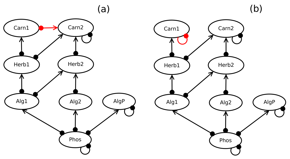
Figure 1: Two versions of the eight-variable lake mesocosm model analyzed by Melbourne-Thomas et al. (2012) and Hosack et al. (2008), and originally presented by Hulot et al. (2000). Abbreviations are: Alg1, edible algae; Alg2, protected algae; AlgP, periphyton; Carn1, invertebrate carnivores; Carn2, fish; Herb1, small herbivores; Herb2, large herbivores; Phos, phosphorus.
The models shown in Figure 1 were created using Dia and so are read using model.dia. Here we assign the two model objects to lake.a and lake.b.
We then simulate for model (a) and use impact.barplot to view simulation outcomes corresponding with observations from the mesocosm experiment (Figure 2).
simlake.a <- system.simulate(1000, lake.a)
impact.barplot(simlake.a)
Doing the same for model (b) gives Figure 3.
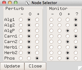
Figure 2: Node selector for the lake mesocosm example.
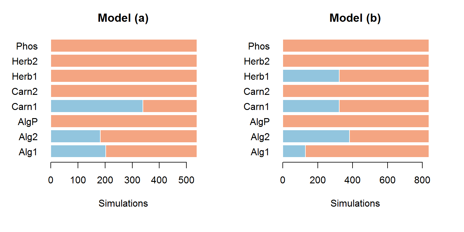
Figure 3: Simulation outcomes from the two lake mesocosm models in response to a positive press perturbation to phosphorous. Each plot shows the fraction of positive (orange), and negative (blue) outcomes at each node. The x-axis indicates the number of simulations (out of 1000 total) that match with the selection for “Monitor” shown in Figure 2.
Approximately 50% of the simulations match with observations for model (a), whereas for model (b) this increases to over 80%. This suggests that model (b) provides a more parsimonious representation of the lake mesocosm system. Melbourne-Thomas et al. (2012) provide a direct comparison of the two models using Bayes factors.
Example II: Antarctic mesocosm
This example is based on experiments conducted at Australia’s Davis Station in Antarctica, which assessed the responses of a natural community of Antarctic marine microbes from near-shore waters to elevated concentrations of CO\(_2\) using environmentally controlled tanks (mesocosms). Davidson et al. (in prep) describe the main components of the Southern Ocean microbial loop represented in these mesocosms and the ecological interactions between them. Specifically:
- Small and large phytoplankton cells consume macronutrients and iron (Fe), although iron is potentially less important for growth of small phytoplankton;
- Small phytoplankton are consumed by heterotrophic nanoflagellates and microzooplankton;
- Large phytoplankton (diatoms) are consumed by microzooplankton;
- Bacteria break down DOC (dissolved organic carbon) and are consumed by heterotrophic nanoflagellates;
- Phytoplankton, microzooplankton and heterotrophic nanoflagellates supply the DOC pool.
These interactions are represented in a model that was built using Dia (black-coloured edges in Figure 4).
When this system was subjected to elevated CO\(_2\) concentrations in experimental mesocosms, the following responses were observed:
- Small phytoplankton increased;
- Large phytoplankton decreased;
- Heterotrophic nanoflagellates decreased; and
- Bacteria increased.
In the model shown in Figure 4 we assume that the direct effects of CO\(_2\) correspond with these observed changes.
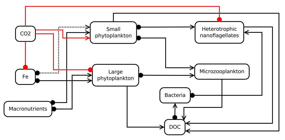
Figure 4: Model (a) representing the effects of CO\(_2\) on the Southern Ocean microbial loop, determined directly from observed responses in experimental mesocosms. These direct effects are shown in red.
We then analyse the response this model to a positive press perturbation to CO\(_2\). In this case we enforce a specific ordering of the nodes, and also enforce self-limitation for each model variable.
labels <- c("CO2", "Fe", "Macronutrients", "Small phytoplankton", "Large phytoplankton",
            "Heterotrophic nanoflagellates", "Microzooplankton", "Bacteria", "DOC")
antarctic.a <- model.dia("Antarctic-a.dia", labels = labels)
antarctic.a <- enforce.limitation(antarctic.a)
As for Example I, we then simulate and use impact.barplot (with the selections shown in Figure 5) to produce Figure 6.
simantarctic.a <- system.simulate(1000, antarctic.a)
impact.barplot(simantarctic.a)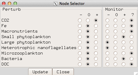
Figure 5: Node selector for the Antarctic mesocosm example..
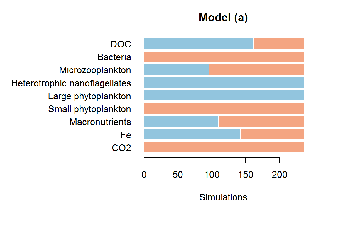
Figure 6: Simulation outcomes in response to a positive press perturbation to CO\(_2\) for Antarctic mesocosm model (a). Each plot shows the fraction of positive (orange), and negative (blue) outcomes at each node.
For this version of the model, less than 20% of the simulations match with our “Monitor” criteria, suggesting that it does not provide a particularly good representation of the Antarctic microbial loop system or its response to increased CO\(_2\) concentrations. Given that increases in dissolved CO\(_2\) are generally expected to have negative impacts of the growth of marine organisms, we could assume a direct negative effect of CO\(_2\) on each of large phytoplankton, small phytoplankton, heterotrophic nanoflagellates, and also the pool of available iron (Figure 7).
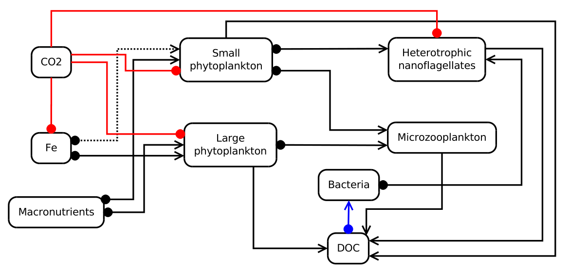
Figure 7: Alternative model (b) representing the effects of CO\(_2\) on the Southern Ocean microbial loop.
Reading this alternative representation from a Dia file
antarctic.b <- model.dia("Antarctic-b.dia", labels = labels)
antarctic.b <- enforce.limitation(antarctic.b)
and exploring simulation outcomes with impact.barplot (with the same “Monitor” criteria as before) produces Figure 8.
simantarctic.b <- system.simulate(1000, antarctic.b)
impact.barplot(simantarctic.b)
In this case, we still only see approximately 20% of simulations that meet our criteria, suggesting that we need to re-think the structure of our model. Davidson et al. (in prep) indicate that bacteria “transform dissolved organic carbon (DOC)… thereby repackaging carbon and making it available to higher trophic levels”. Looking at our original model, we haven’t quite captured this in our representation of interactions between bacteria, DOC and macronutrients. In a third version of our microbial loop model (model (c) — Figure 9) we therefore assume a negative effect of bacteria on DOC and a positive effect of bacteria on macronutrients (which includes carbon).
Reading a third Dia version of the model
antarctic.c <- model.dia("Antarctic-c.dia", labels = labels)
antarctic.c <- enforce.limitation(antarctic.c)
and repeating the simulation and impact.barplot steps from above gives Figure 10.
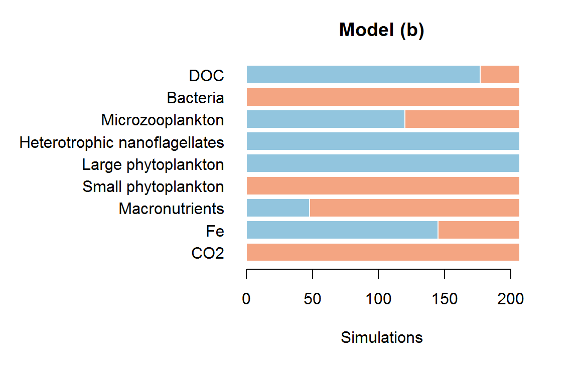
Figure 8: Simulation outcomes in response to a positive press perturbation to the CO\(_2\) for the alternative microbial loop model (b) shown in Figure 7.

Figure 9: Alternative model (c) representing the effects of CO\(_2\) on the Southern Ocean microbial loop.
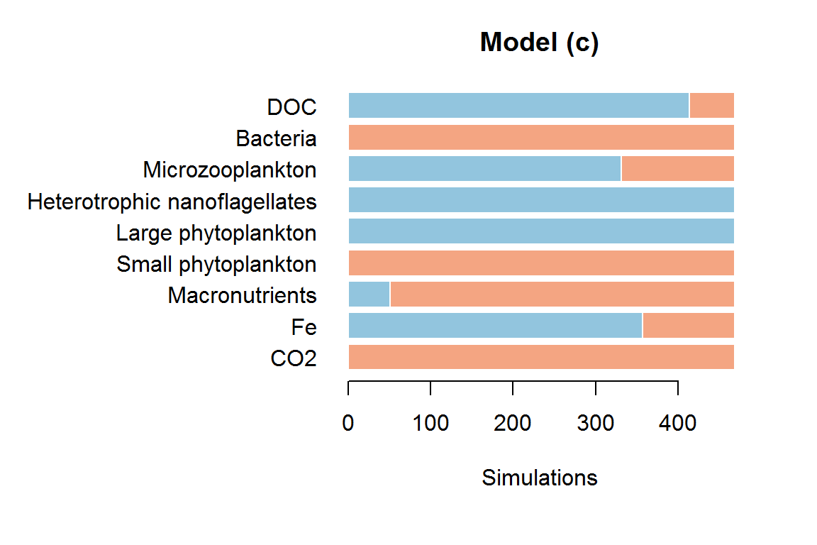
Figure 10: Simulation outcomes in response to a positive press perturbation to the CO\(_2\) for the alternative microbial loop model (c) shown in Figure 9.
References
Hosack, Geoffrey R, Keith R Hayes, and Jeffrey M Dambacher. 2008. “Assessing model structure uncertainty through an analysis of system feedback and Bayesian networks.” Ecological Applications 18 (4): 1070–82.
Hulot, F D, G Lacroix, F Lescher-Moutoué, and M Loreau. 2000. “Functional diversity governs ecosystem response to nutrient enrichment.” Nature 405 (May): 340–44.
Melbourne-Thomas, J, S Wotherspoon, B Raymond, and A Constable. 2012. “Comprehensive Evaluation of Model Uncertainty in Qualitative Network Analyses.” Ecological Monographs 82 (4). Eco Soc America: 505–19.